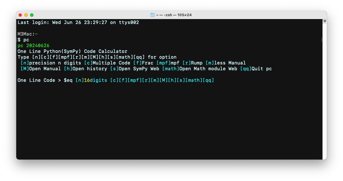
ターミナル立ち上げてすぐに数式を入力できる
数値計算・代数計算にとって強力な助っ人SymPyをもっと簡単に
Pythonは素晴らしい言語です
SymPyライブラリは数学の強力助っ人
でも使うためにはいくつものお膳立てが必要
ターミナルにコマンドpcを打ち込むだけでPython一行コードを即入力・即出力を可能にします
Pythonを立ち上げる必要なし
Pythonのコーディングも必要なし
SymPyライブラリのインポートはじめお膳立ても必要なし
シェルスクリプトは1つpc.shだけだから設置が容易
3ステップで高度な数学計算ができる
1.ターミナルを立ち上げる
2.コマンドpcを打ち込む
3.数式 expand((x+y+z)**3)を入力

【更新】
20240626
・マニュアルを拡充
SymPyに加え-math — 数学関数-を追加
・オプションに
[math]Open Math module Web
を追加
python標準モジュールmath
math module Doc Web表示
20230908
・インストールするファイルを1つだけにした
・モードを9つにした
・出力を7つにした
・カラー表示にした
・複数行コード入力メニュー[2c]Codeを追加
【動作確認環境】
【macOS14.5】
M3Mac
Python 3.11.9
zsh
【macOS12.6.5】
Python 3.11.4
Bash、zsh
【Ubuntu22.04.2LTS】
Python 3.11.1
Bash
【必須Pythonライブラリ】
SymPyライブラリ
mpmathライブラリ
【インストール】
HOMEにディレクトリmyscript/pcをつくる
HOME/myscript/pcに
py.sh
を配置
もし設置するディレクトリを変更する場合
変数PCDIRを変更
# pc.sh
# pc.shの設置ディレクトリ
PCDIR=$HOME/myscript/pc
MacOS .zshrcに以下を追記
# .zshrc
source $HOME/myscript/pc/pc.sh
ubuntu .bashrcに以下を追記
# .bashrc
alias open=xdg-open
source $HOME/myscript/pc/pc.sh
【OPTION】
[n] set precision n digits (default:16 digits)
[c] Enter multiple Code TAB OK Press ‘##’ to Stop inputting
[f] 2/3 -> Fraction(“2/3”).limit_denominator()
[mpf] 3.14 -> mpf(“3.14”) mp(multiple-precision)f(Real float)
[r] verify Rumps example
[m] less manual This manual page Press ‘q’ to stop
[M] open manual
[h] open history open $PCDIR/pchistory.txt
[s] open SymPy Web Site
[math] Open Math module Web
[qq] quit pc
【OUTPUT】
[1]pprint(eq,use_unicode=False)
[2]pprint(eq,use_unicode=True)
[3]pprint(eval(eq))
[4]print(eval(eq))
[5]N(eq, precision)
[6]latex(eval(eq))
[7]latex(N(eq,precision))
シェルスクリプト pc.sh
#!/usr/bin/env bash

# pc
# -- One Line Python(SymPy) Code Calculator --

pcversion='20240626'

# Select Color Set
# Terminal Back Color : Black (Font Color : White)
blue='\033[94m';violet='\033[95m';green='\033[92m';mizu='\033[96m';red='\033[91m';yellow='\033[93m'

# Terminal Back Color : White (Font Color : Black)
# blue='\033[1;30m';violet='\033[1;30m';green='\033[1;30m';mizu='\033[1;30m'

# pc.shの設置ディレクトリ
PCDIR=HOME/myscript/pc

# コマンド pce
# pc.sh 編集
function pce(){
openPCDIR/pc.sh
}

# コマンド pcl
# 入力履歴表示
function pcl(){
open PCDIR/pchistory.txt
}

# コマンド pcd
# SymPy Doc Web表示
function pcd(){
open 'https://docs.sympy.org/latest/tutorials/intro-tutorial/features.html'
}

# コマンド pcmath
# math module Doc Web表示
function pcmath(){
open 'https://docs.python.org/ja/3/library/math.html'
}


# コマンド help
function helppc(){
echo -e "helptxt" | less -R -X
}

# コマンド helpe Manual外部エディターに表示
function helpe(){
echo -e "helptxt" | sed -e 's%[[]9[2-6]m%%g' -e 's%[[]1;30m%%g' -e 's%[[]0m%%g' -e 's%[[]m%%g'>PCDIR/help.txt
open PCDIR/help.txt
}


# Manual TEXT
helptxt=(cat << EOF
General Commands Manual
NAME
   pc -  One Line Python(SymPy) Code Calculator

SYNTAX
   pc

VERSION
   This man page documents pc version {pcversion}

Copyright 2023 sakurAi Science Factory, Inc.
This is free software with ABSOLUTELY NO WARRANTY.

Recommended Terminal Font
Ubuntu Mono

DESCRIPTION
Enter One Line Code>\$eq [n]16digits [c][f][mpf][r][m][M][h][s][qq]
One Line Python(SymPy) Code
you can use '^' instead of '**'

IMPORT LIBRARY・MODULE
import math
from fractions import Fraction as Frac
from mpmath import *
from pprint import pprint
mp.pretty = True
from sympy import *
from spb import *  # SymPy Plotting Backends (SPB)
import japanize_matplotlib
import matplotlib.pyplot as plt

init_printing() #降べきの順
# init_printing(order='rev-lex') #昇べきの順
var('a:z')
f = Function('f')


OPTION
[n] set precision n digits (default:16 digits)
[c] Enter multiple Code     TAB OK  Press '##' to Stop inputting
[f] 2/3 -> Fraction("2/3").limit_denominator()
[mpf] 3.14 -> mpf("3.14")  mp(multiple-precision)f(Real float)
[r] verify Rumps example
[m] less manual  This manual page   Press 'q' to stop
[M] open manual
[h] open history   open \$PCDIR/pchistory.txt
[s] open SymPy Web Site
[math] Open Math module Web
[qq] quit pc

OUTPUT  One Line Python(SymPy) Code [f]Frac [mpf]mpf
[1]pprint(eq,use_unicode=False)
[2]pprint(eq,use_unicode=True)
[3]pprint(eval(eq))
[4]print(eval(eq))
[5]N(eq, precision)
[6]latex(eval(eq))
[7]latex(N(eq,precision))

OUTPUT  [c]multiple Code
[8]exec('eq')

[EXPRESSION] All SymPy Code OK{blue}────────────────────────────────────────────────────────────────────
{violet}Math\033[0m
SymPy Code{green}OUTPUT\033[0m


{mizu}-BASIC-\033[0m{blue}────────────────────────────────────────────────────────────────────
{violet}algebra symbolic variable\033[0m
from a to z{blue}────────────────────────────────────────────────────────────────────
{violet}algebra symbolic function\033[0m
default only f
x, y = symbols('x y', positive=True)
a, b = symbols('a b', real=True){blue}────────────────────────────────────────────────────────────────────
{violet}Natural Representation\033[0m
print(expand((x+y)**2)){green}x**2 + 2*x*y + y**2\033[0m

pprint(expand((x+y)**2))
{green} 2            2{green}x  + 2⋅x⋅y + y \033[0m

{blue}────────────────────────────────────────────────────────────────────{violet}substitution\033[0m
(x^2+x+1).subs(x, 1)
{green}3\033[0m{blue}────────────────────────────────────────────────────────────────────
{violet}quotient\033[0m
13 // 5{green}2\033[0m

{blue}────────────────────────────────────────────────────────────────────{violet}remainder\033[0m
13 % 5
{green}3\033[0m{blue}────────────────────────────────────────────────────────────────────
{violet}quotient and remainder\033[0m
divmod(25, 3){green}(8, 1)\033[0m

{blue}────────────────────────────────────────────────────────────────────{violet}fraction\033[0m
2/3
{green}0.6666666666666666\033[m

Frac(2,3){green}2/3\033[m

Frac("2/3")
{green}6004799503160661/9007199254740992\033[m

Frac("2/3").limit_denominator(){green}2/3\033[m

[c]Code
pprint(Frac("2/3")+Frac("1/7"))
{green}17{green}──
{green}21\033[m

[f]Frac
2/3+1/7{green}17
{green}──{green}21\033[0m


{mizu}-NUMBER-\033[0m{blue}────────────────────────────────────────────────────────────────────
{violet}Pi\033[0m
pi{green}3.141592653589793 (default 16digits)\033[0m

{blue}────────────────────────────────────────────────────────────────────{violet}Napier Constant\033[0m
E
{green}2.718281828459045 (default 16digits)\033[0m{blue}────────────────────────────────────────────────────────────────────
{violet}imaginary unit\033[0m
(2+3j)*(5-7j){green}(31+1j)
{green}31.0 + 1.0⋅ⅈ\033[0m{blue}────────────────────────────────────────────────────────────────────
{violet}imaginary unit(SymPy)\033[0m
exp(cos(E**I)+sin(E*pi)){green}    ⎛ ⅈ⎞
{green} cos⎝ℯ ⎠ + sin(ℯ⋅π){green}ℯ

{green}6.237024243670621 - 3.292937458733587⋅ⅈ\033[0m

I**I{green} ⅈ
{green}ⅈ{green}0.2078795763507619\033[0m

{blue}────────────────────────────────────────────────────────────────────{violet}Degree\033[0m
mp.degree
{green}0.0174532925199433\033[0m

pi/180{green}0.01745329251994330\033[0m

{blue}────────────────────────────────────────────────────────────────────{violet}Golden Ratio\033[0m
phi
{green}1.618033988749895\033[0m{blue}────────────────────────────────────────────────────────────────────
{violet}Euler's constant Gamma\033[0m
mp.euler{green}0.5772156649015329\033[0m

{blue}────────────────────────────────────────────────────────────────────{violet}Catalan’s constant\033[0m
mp.catalan
{green}0.915965594177219\033[0m{blue}────────────────────────────────────────────────────────────────────
{violet}Khinchin’s constant\033[0m
mp.khinchin{green}2.685452001065306\033[0m

{blue}────────────────────────────────────────────────────────────────────{violet}Glaisher’s constant\033[0m
mp.glaisher
{green}1.282427129100623\033[0m{blue}────────────────────────────────────────────────────────────────────
{violet}Mertens constant\033[0m
mp.mertens{green}0.2614972128476428\033[0m

{blue}────────────────────────────────────────────────────────────────────{violet}Twin prime constant\033[0m
mp.twinprime
{green}0.6601618158468696\033[0m{mizu}-FUNCTION-\033[0m
{blue}────────────────────────────────────────────────────────────────────{violet}square root\033[0m
sqrt(2)
{green}1.414213562373095 (default 16digits)\033[0m{blue}────────────────────────────────────────────────────────────────────
{violet}LCM (Least Common Multiple)\033[0m
lcm(120, 99){green}3960\033[0m

{blue}────────────────────────────────────────────────────────────────────{violet}GCD (Greatest Common Divisor)\033[0m
gcd(12, 18)
{green}6\033[0m{blue}────────────────────────────────────────────────────────────────────
{violet}trigonometry\033[0m
sin(pi/3){green}  ___
{green}\/ 3{green}-----
{green} 2  \033[0m

sin(radians(60)){green}0.8660254037844387\033[0m

degrees(pi/3).evalf()
{green}60.0000000000000\033[0m

asin()
sinh()
asinh(){blue}────────────────────────────────────────────────────────────────────
{violet}exponential\033[0m
exp(1){green}e
{green}ℯ{green}E
{green}2.718281828459045\033[0m{blue}────────────────────────────────────────────────────────────────────
{violet}natural logarithm\033[0m
log(E**2){green}2\033[0m

{blue}────────────────────────────────────────────────────────────────────{violet}common lagarithm\033[0m
log(2,10)  log(x, base)
{green}log(2)/log(10){green}0.3010299956639812\033[0m

{blue}────────────────────────────────────────────────────────────────────{violet}gamma function\033[0m
gamma(4)
{green}6\033[0m
gamma(sqrt(2)){green}0.8865814287192591\033[0m

{blue}────────────────────────────────────────────────────────────────────{violet}binomial\033[0m
binomial(5,2)
{green}10\033[0m
binomial(n,3){green}⎛n⎞
{green}⎜ ⎟{green}⎝3⎠\033[0m

{blue}────────────────────────────────────────────────────────────────────{violet}permutation\033[0m
math.perm(5,2)
{green}20\033[0m{blue}────────────────────────────────────────────────────────────────────
{violet}combination\033[0m
math.comb(5,2){green}10\033[0m

{blue}────────────────────────────────────────────────────────────────────{violet}absolute value\033[0m
abs(-3)
{green}3\033[0m{blue}────────────────────────────────────────────────────────────────────
{violet}prime factorization\033[0m
factorint(60){green}{2: 2, 3: 1, 5: 1}\033[0m

{blue}────────────────────────────────────────────────────────────────────{violet}factorial\033[0m
factorial(10)
{green}3628800\033[0m{blue}────────────────────────────────────────────────────────────────────
{violet}KroneckerDelta\033[0m
KroneckerDelta(1, 2){green}0\033[0m

KroneckerDelta(i, j)
{green}δ{green} i,j\033[0m

{blue}────────────────────────────────────────────────────────────────────{violet}besseli\033[0m
besselj(n, z).diff(z)
{green}besselj(n - 1, z)   besselj(n + 1, z){green}───────────────── - ─────────────────
{green}        2                   2        \033[0m

besselj(n, z).rewrite(jn){green}√2⋅√z⋅jn(n - 1/2, z)
{green}────────────────────{green}         √π         \033[0m


{mizu}-SIMPILIFICATION-\033[0m{blue}────────────────────────────────────────────────────────────────────
{violet}simplify\033[0m
simplify(cos(x)**2+sin(x)**2){green}1\033[0m

(x**2 + 2*x + 1)/(x**2 + x)
{green} 2{green}x  + 2⋅x + 1
{green}────────────{green}    2
{green}   x  + x \033[0m

simplify((x**2 + 2*x + 1)/(x**2 + x)){green}x + 1
{green}─────{green}  x \033[0m

{blue}────────────────────────────────────────────────────────────────────{violet}expand\033[0m
expand((x+y+z)**3)
{green} 3      2        2          2                  2    3      2          2    3{green}x  + 3⋅x ⋅y + 3⋅x ⋅z + 3⋅x⋅y  + 6⋅x⋅y⋅z + 3⋅x⋅z  + y  + 3⋅y ⋅z + 3⋅y⋅z  + z \033[0m

{blue}────────────────────────────────────────────────────────────────────{violet}factor\033[0m
factor(a^8-b^8)
{green}                ⎛ 2    2⎞ ⎛ 4    4⎞{green}(a - b)⋅(a + b)⋅⎝a  + b ⎠⋅⎝a  + b ⎠\033[0m

{blue}────────────────────────────────────────────────────────────────────{violet}collec\033[0m
x*y^2+3*x^3*y+5*x*y-7*x^3*y^2
{green}     3  2      3        2{green}- 7⋅x ⋅y  + 3⋅x ⋅y + x⋅y  + 5⋅x⋅y\033[0m

collect(x*y^2+3*x^3*y+5*x*y-7*x^3*y^2, x)
{green} 3 ⎛     2      ⎞     ⎛ 2      ⎞{green}x ⋅⎝- 7⋅y  + 3⋅y⎠ + x⋅⎝y  + 5⋅y⎠\033[0m

collect(x*y^2+3*x^3*y+5*x*y-7*x^3*y^2, y)
{green} 2 ⎛     3    ⎞     ⎛   3      ⎞{green}y ⋅⎝- 7⋅x  + x⎠ + y⋅⎝3⋅x  + 5⋅x⎠\033[0m

{blue}────────────────────────────────────────────────────────────────────{violet}cancel\033[0m
(x**2 + 2*x + 1)/(x**2 + x)
{green} 2{green}x  + 2⋅x + 1
{green}────────────{green}    2
{green}   x  + x   \033[0m

cancel((x**2 + 2*x + 1)/(x**2 + x)){green}x + 1
{green}─────{green}  x \033[0m

{blue}────────────────────────────────────────────────────────────────────{violet}apart\033[0m
1/((x-1)*(x+1))
{green}       1{green}───────────────
{green}(x - 1)⋅(x + 1)\033[0m

apart(1/((x-1)*(x+1))){green}      1           1
{green}- ───────── + ─────────{green}  2⋅(x + 1)   2⋅(x - 1)\033[0m

{blue}────────────────────────────────────────────────────────────────────{violet}separatevars\033[0m
(x*y)**y
{green}     y{green}(x⋅y) \033[0m

separatevars((x*y)**y, force=True)
{green} y  y{green}x ⋅y \033[0m

x*y*z*sin(x)*cos(x)+x^2*y*z^3*cos(x)
{green} 2    3{green}x ⋅y⋅z ⋅cos(x) + x⋅y⋅z⋅sin(x)⋅cos(x)\033[0m

separatevars(x*y*z*sin(x)*cos(x)+x^2*y*z^3*cos(x))
{green}      ⎛            2⎞{green}x⋅y⋅z⋅⎝sin(x) + x⋅z ⎠⋅cos(x)\033[0m

{blue}────────────────────────────────────────────────────────────────────{violet}ratsimp\033[0m
reduce fractions to a common denominator

ratsimp(1/x + 1/y)
{green}x + y{green}─────
{green} x⋅y \033[0m{blue}────────────────────────────────────────────────────────────────────
{violet}radsimp\033[0m
Rationalize the denominator by removing square roots

1/(1 + sqrt(2) + sqrt(3) + sqrt(5)){green}       1
{green}────────────────{green}1 + √2 + √3 + √5\033[0m

radsimp(1/(1 + sqrt(2) + sqrt(3) + sqrt(5)))
{green}-34⋅√10 - 26⋅√15 - 55⋅√3 - 61⋅√2 + 14⋅√30 + 93 + 46⋅√6 + 53⋅√5{green}──────────────────────────────────────────────────────────────
{green}                              71                              \033[0m{blue}────────────────────────────────────────────────────────────────────
{violet}expand_trig\033[0m
expand_trig(sin(x + y)){green}sin(x)⋅cos(y) + sin(y)⋅cos(x)\033[0m

{blue}────────────────────────────────────────────────────────────────────{violet}trigsimp\033[0m
trigsimp(sin(x)*cos(y) + sin(y)*cos(x))
{green}sin(x + y)\033[0m{blue}────────────────────────────────────────────────────────────────────
{violet}expand_log\033[0m
expand_log(log(x*y), force=True){green}log(x) + log(y)\033[0m

{blue}────────────────────────────────────────────────────────────────────{violet}logcombine\033[0m
logcombine(log(x) + log(y), force=True)
{green}log(x⋅y)\033[0m{blue}────────────────────────────────────────────────────────────────────
{violet}powsimp\033[0m
x**a*x**b{green} a  b
{green}x ⋅x \033[0m

powsimp(x**a*x**b){green} a + b
{green}x     \033[0m{blue}────────────────────────────────────────────────────────────────────
{violet}expand_power_exp\033[0m
3**(y + 2){green} y + 2
{green}3     \033[0m

expand_power_exp(3**(y + 2)){green}   y
{green}9⋅3 \033[0m

pprint(expand_power_exp(Symbol('x', zero=False)**(y + 2))){green} 2  y
{green}x ⋅x \033[0m{blue}────────────────────────────────────────────────────────────────────
{violet}expand_power_base\033[0m
(x*y)**z{green}     z
{green}(x⋅y) \033[0m

expand_power_base((x*y)**z, force=True){green} z  z
{green}x ⋅y \033[0m{blue}────────────────────────────────────────────────────────────────────
{violet}powdenest\033[0m
(x**a)**b{green}    b
{green}⎛ a⎞{green}⎝x ⎠ \033[0m

powdenest((x**a)**b, force=True)
{green} a⋅b{green}x   \033[0m

{blue}────────────────────────────────────────────────────────────────────{violet}expand_func\033[0m
expand_func(gamma(x+3))
{green}x⋅(x + 1)⋅(x + 2)⋅Γ(x)\033[0m

expand_func(binomial(n,3)){green}n⋅(n - 2)⋅(n - 1)
{green}─────────────────{green}        6        \033[0m

{blue}────────────────────────────────────────────────────────────────────{violet}FUNCsimp\033[0m
gammasimp(gamma(x)*gamma(1-x))
{green}   π{green}────────
{green}sin(π⋅x)c

combsimp(binomial(n+2,k)/binomial(n,k)){green}    (n + 1)⋅(n + 2)
{green}───────────────────────{green}(k - n - 2)⋅(k - n - 1)\033[0m

kroneckersimp( 1+KroneckerDelta(0, j) * KroneckerDelta(1, j))
{green}1\033[0m

besselsimp(z*besseli(0, z) + z*(besseli(2, z))/2 + besseli(1, z)){green}3⋅z⋅besseli(0, z)
{green}─────────────────{green}        2        \033[0m

hypersimp(factorial(n)**2 / factorial(2*n), n)
{green}   n + 1{green}───────────
{green}2⋅(2⋅n + 1)\033[0m{blue}────────────────────────────────────────────────────────────────────
{violet}.rewrite\033[0m
tan(x).rewrite(sin){green}     2
{green}2⋅sin (x){green}─────────
{green} sin(2⋅x)\033[0m

(cos(x)).rewrite(sin){green}   ⎛    π⎞
{green}sin⎜x + ─⎟{green}   ⎝    2⎠\033[0m

factorial(x).rewrite(gamma)
{green}Γ(x + 1)\033[0m{mizu}-SEQUENCE-\033[0m
{blue}────────────────────────────────────────────────────────────────────{violet}sequence\033[0m
sequence(k**2,(k,1,10))
{green}[1, 4, 9, 16, …]\033[0m

sequence(k**2,(k,1,10))[9]{green}100\033[0m

{blue}────────────────────────────────────────────────────────────────────{violet}summation of a sequence\033[0m
Sum(k**2,(k,1,n))
{green}  n{green} ___
{green} ╲{green}  ╲    2
{green}  ╱   k{green} ╱
{green} ‾‾‾{green}k = 1  \033[0m

Sum(k**2,(k,1,n)).doit()
{green} 3    2{green}n    n    n
{green}── + ── + ─{green}3    2    6\033[0m

{blue}────────────────────────────────────────────────────────────────────{violet}product of a sequence\033[0m
Product(k,(k,1,10))
{green}  10{green}─┬─┬─
{green} │ │  k{green} │ │
{green}k = 1  \033[0m

product(k,(k,1,10)){green}3628800\033[0m

{blue}────────────────────────────────────────────────────────────────────{violet}Seki-Bernoulli number\033[0m
bernoulli(1)
{green}1/2\033[0m

bernoulli(2){green}1/6\033[0m


{mizu}-EQUATION-\033[0m{blue}────────────────────────────────────────────────────────────────────
{violet}Eq\033[0m
Eq(x^3, x^2-1){green} 3    2
{green}x  = x  - 1\033[0m{blue}────────────────────────────────────────────────────────────────────
{violet}solve\033[0m
solve(x^2+x+4){green}⎡  1   √15⋅ⅈ    1   √15⋅ⅈ⎤
{green}⎢- ─ - ─────, - ─ + ─────⎥{green}⎣  2     2      2     2  ⎦\033[0m

solve(a*x**2+b*x+c, x)
{green}⎡        _____________          _____________⎤{green}⎢       ╱           2          ╱           2 ⎥
{green}⎢-b - ╲╱  -4⋅a⋅c + b    -b + ╲╱  -4⋅a⋅c + b  ⎥{green}⎢─────────────────────, ─────────────────────⎥
{green}⎣         2⋅a                    2⋅a         ⎦\033[0m

solve(x**2-1,x)[0]{green}-1\033[0m

[f]Frac
solve([2/3*x-y-1,3/7*x-2*y-5/9],[x,y])
{green}⎧   91      11⎫{green}⎨x: ──, y: ───⎬
{green}⎩   57     171⎭\033[0m

solve([x+y-4,x-y-2],[x,y]){green}{x: 3, y: 1}\033[0m

list(solve([x+y-4,x-y-2]).items())[0]
{green}(x, 3)\033[0m

list(solve([x+y-4,x-y-2],[x,y]).items())[0][1]{green}3\033[0m

{blue}────────────────────────────────────────────────────────────────────{violet}dsolve\033[0m
variable function f
Eq(Derivative(f(t),t,2)-f(t),exp(t))
{green}  2{green} d                  t
{green}───(f(t)) - f(t) = ℯ{green}  2
{green}dt                   \033[0m

dsolve(Eq(f(t).diff(t, 2) - f(t), exp(t)), f(t)){green}           -t   ⎛     t⎞  t
{green}f(t) = C₂⋅ℯ   + ⎜C₁ + ─⎟⋅ℯ{green}                ⎝     2⎠   \033[0m

dsolve(Eq(f(t).diff(t, 2) - f(t), exp(t)), f(t), ics={f(0):1, f(t).diff(t,1).subs(t, 0):1})
{green}                     -t{green}       ⎛t   3⎞  t   ℯ
{green}f(t) = ⎜─ + ─⎟⋅ℯ  + ───{green}       ⎝2   4⎠       4 \033[0m


{mizu}-CALCULUS-\033[0m{blue}────────────────────────────────────────────────────────────────────
{violet}differential\033[0m
diff(x^3+x^2+x+1){green}   2
{green}3⋅x  + 2⋅x + 1\033[0m

diff(sin(x),x,3){green}-cos(x)\033[0m

Derivative(exp(x**2),x,3)
{green}  3⎛ ⎛ 2⎞⎞{green} d ⎜ ⎝x ⎠⎟
{green}───⎝ℯ    ⎠{green}  3
{green}dx        \033[0m

Derivative(exp(x**2),x,3).doit(){green}                ⎛ 2⎞
{green}    ⎛   2    ⎞  ⎝x ⎠{green}4⋅x⋅⎝2⋅x  + 3⎠⋅ℯ    \033[0m

[c]Code
f = Function('f')
g = Function('g')
eq = (f(x) * g(x)).diff(x)
pprint(eq)
{green}     d               d{green}f(x)⋅──(g(x)) + g(x)⋅──(f(x))
{green}     dx              dx      \033[0m{blue}────────────────────────────────────────────────────────────────────
{violet}indefinite integral\033[0m
integrate(3*x^2+2*x+1){green} 3    2
{green}x  + x  + x\033[0m

[f]Frac
Integral(3*x^2+2*x-2/3){green}⌠
{green}⎮ ⎛   2         2⎞{green}⎮ ⎜3⋅x  + 2⋅x - ─⎟ dx
{green}⎮ ⎝             3⎠{green}⌡                    \033[0m

[f]Frac
Integral(3*x^2+2*x-2/3).doit()
{green} 3    2   2⋅x{green}x  + x  - ───
{green}           3 \033[0m{violet}definite integral\033[0m
integrate(x**3,(x,0,1))
{green}1/4\033[0m

[f]Frac
Integral(2/3*x^5, (x, 0, 2/3)){green}2/3
{green} ⌠{green} ⎮     5
{green} ⎮  2⋅x{green} ⎮  ──── dx
{green} ⎮   3{green} ⌡
{green} 0         \033[0m

[f]Frac
Integral(2/3*x^5, (x, 0, 2/3)).doit(){green} 64
{green}────{green}6561\033[0m

{blue}────────────────────────────────────────────────────────────────────{violet}Taylor series\033[0m
series(sin(x),x, 0, 12)
{green}     3     5     7       9        11{green}    x     x     x       x        x         ⎛ 12⎞
{green}x - ── + ─── - ──── + ────── - ──────── + O⎝x  ⎠{green}    6    120   5040   362880   39916800         \033[0m

{violet}Taylor series coefficient list\033[0m
taylor(sin, 0, 5){green}[0.0, 1.0, 0.0, -0.1666666666666667, 0.0, 0.008333333333333333]\033[0m

series(sin(x),x, 0, 12).removeO()
{green}     3     5     7       9        11{green}    x     x     x       x        x
{green}x - ── + ─── - ──── + ────── - ────────{green}    6    120   5040   362880   39916800\033[0m

series(sin(x),x, 0, 12).removeO().subs(x,1)
{green}0.8414709846480680\033[0m{mizu}-INFINITY-\033[0m
{blue}────────────────────────────────────────────────────────────────────{violet}infinity\033[0m
oo
{green}∞\033[0m

Integral(1/(1+x**2), (x, -oo, oo)){green}∞
{green}⌠{green}⎮    1
{green}⎮  ────── dx{green}⎮   2
{green}⎮  x  + 1{green}⌡
{green}-∞          \033[0m

Integral(1/(1+x**2), (x, -oo, oo)).doit(){green}π\033[0m

integrate(1/(1+x**2), (x, -oo, oo))
{green}π\033[0m{mizu}-LIMIT-\033[0m
{blue}────────────────────────────────────────────────────────────────────{violet}limit\033[0m
limit(sin(x)/x, x, 0)
{green}1\033[0m

Limit((x^2+x-1)/(2*x^2-x+2), x, oo){green}    ⎛  2         ⎞
{green}    ⎜ x  + x - 1 ⎟{green}lim ⎜────────────⎟
{green}x─→∞⎜   2        ⎟{green}    ⎝2⋅x  - x + 2⎠\033[0m

Limit((x^2+x-1)/(2*x^2-x+2), x, oo).doit()
{green}1/2\033[0m

limit((x^2+x-1)/(2*x^2-x+2), x, oo){green}1/2\033[0m

limit(tan(x), x, pi/2, '+')
{green}-∞\033[0m

limit(tan(x), x, pi/2, '-'){green}∞\033[0m


{mizu}-MATRIX-\033[0m{blue}────────────────────────────────────────────────────────────────────
{violet}Matrix\033[0m
Matrix([[1, 2], [2, 2]]){green}⎡1  2⎤
{green}⎢    ⎥{green}⎣2  2⎦\033[0m

Matrix([[1, 2], [2, 2]])**2
{green}⎡5  6⎤{green}⎢    ⎥
{green}⎣6  8⎦\033[0m

eye(3){green}⎡1  0  0⎤
{green}⎢       ⎥{green}⎢0  1  0⎥
{green}⎢       ⎥{green}⎣0  0  1⎦\033[0m

zeros(3)
{green}⎡0  0  0⎤{green}⎢       ⎥
{green}⎢0  0  0⎥{green}⎢       ⎥
{green}⎣0  0  0⎦\033[0m

ones(3){green}⎡1  1  1⎤
{green}⎢       ⎥{green}⎢1  1  1⎥
{green}⎢       ⎥{green}⎣1  1  1⎦\033[0m

diag(1, 2, 3)
{green}⎡1  0  0⎤{green}⎢       ⎥
{green}⎢0  2  0⎥{green}⎢       ⎥
{green}⎣0  0  3⎦\033[0m{blue}────────────────────────────────────────────────────────────────────
{violet}A.det()\033[0m
Matrix([[1, 2], [2, 2]]).det(){green}-2\033[0m

{blue}────────────────────────────────────────────────────────────────────{violet}A.inv()\033[0m
Matrix([[1, 2], [2, 2]]).inv()
{green}⎡-1   1  ⎤{green}⎢        ⎥
{green}⎣1   -1/2⎦\033[0m

Matrix([[1, 2], [2, 2]])**(-1){green}⎡-1   1  ⎤
{green}⎢        ⎥{green}⎣1   -1/2⎦\033[0m

{blue}────────────────────────────────────────────────────────────────────{violet}A.adjugate()\033[0m
Matrix([[1, 2], [3, 4]]).adjugate()
{green}⎡4   -2⎤{green}⎢      ⎥
{green}⎣-3  1 ⎦\033[0m{blue}────────────────────────────────────────────────────────────────────
{violet}A.transpose()\033[0m
Matrix([[1, 2], [3, 4]]).transpose(){green}⎡1  3⎤
{green}⎢    ⎥{green}⎣2  4⎦\033[0m

{blue}────────────────────────────────────────────────────────────────────{violet}A.rank()\033[0m
Matrix([[1, 2, 3], [4, 5, 0], [0, 0, 0]]).rank()
{green}2\033[0m{blue}────────────────────────────────────────────────────────────────────
{violet}A.eigenvals()\033[0m
Matrix([[1, 2], [2, 2]]).eigenvals(){green}⎧3   √17     3   √17   ⎫
{green}⎨─ - ───: 1, ─ + ───: 1⎬{green}⎩2    2      2    2    ⎭\033[0m

{blue}────────────────────────────────────────────────────────────────────{violet}A.eigenvects()\033[0m
Matrix([[1, 2], [2, 2]]).eigenvects()
{green}⎡⎛            ⎡⎡  √17   1⎤⎤⎞  ⎛            ⎡⎡  1   √17⎤⎤⎞⎤{green}⎢⎜3   √17     ⎢⎢- ─── - ─⎥⎥⎟  ⎜3   √17     ⎢⎢- ─ + ───⎥⎥⎟⎥
{green}⎢⎜─ - ───, 1, ⎢⎢   4    4⎥⎥⎟, ⎜─ + ───, 1, ⎢⎢  4    4 ⎥⎥⎟⎥{green}⎢⎜2    2      ⎢⎢         ⎥⎥⎟  ⎜2    2      ⎢⎢         ⎥⎥⎟⎥
{green}⎣⎝            ⎣⎣    1    ⎦⎦⎠  ⎝            ⎣⎣    1    ⎦⎦⎠⎦\033[0m{mizu}-ZETA-\033[0m
{blue}────────────────────────────────────────────────────────────────────{violet}zeta\033[0m
zeta(2)
{green} 2{green}π
{green}──{green}6 \033[0m

zeta(-1)
{green}-1/12\033[0m{blue}────────────────────────────────────────────────────────────────────
{violet}zetazero\033[0m
zetazero(1){green}(0.5 + 14.13472514173469j)\033[0m


{mizu}-Boolean-valued check-\033[0m{blue}────────────────────────────────────────────────────────────────────
{violet}==\033[0m
1+1 == 3{green}False\033[0m

expand((x+y)**2) == x**2+2*x*y+y**2
{green}True\033[0m{mizu}-mpmath floating-point-\033[0m
{blue}────────────────────────────────────────────────────────────────────
(-2)**mpf("0.5"){green}(0.0 + 1.4142135623730950488016887242096980785696718753769j)\033[0m


{mizu}-PLOT-\033[0m{blue}────────────────────────────────────────────────────────────────────
{violet}from spb import *  # SymPy Plotting Backends (SPB)\033[0m{violet}import japanize_matplotlib\033[0m
{violet}import matplotlib.pyplot as plt\033[0m

plot(sin(x), (x, 0, 7), ylabel = "y")

graphics(line(sin(x)),axis_center="auto", grid=False)

p1 = plot_list([2], [4],
legend=True,
is_point = True,
line_color = "red",
show = False)
p2 = plot(x**2, (x, 0, 3),
line_color = "blue",
show = False)
(p1+p2).show()

f1 = x
f2 = x**2
f3 = sin(x)
plot((f1,"1次関数"), (f2, "2次関数"),(f3,"三角関数"),
(x, 0, 4),
rendering_kw=[{"color":"red"},{"color":"blue"},{"color":"green"}],
backend=MB,  # Choromeブラウザー出力
title = "backend=MB (MatplotlibBackend)",
axis_center="auto",
grid=True,
xlabel = "x",
ylabel = "y")

f1 = x
f2 = x**2
f3 = sin(x)
plot((f1,"1次関数"), (f2, "2次関数"),(f3,"三角関数"),
(x, -2, 2),
backend=BB,  # Choromeブラウザー出力
title = "backend=BB (BokehBackend)",
xlabel = "x",
ylabel = "y")

f1 = x
f2 = x**2
f3 = sin(x)
plot((f1,"1次関数"), (f2, "2次関数"),(f3,"三角関数"),
(x, -2, 2),
backend=PB,  # Choromeブラウザー出力
title = "backend=PB (PlotyBackend)",
xlabel = "x",
ylabel = "y")

p = plot(sin(x), (x, -pi, pi), ylabel="sin x", axis_center="auto",backend=MB, show=False)
ax = p.ax
ax.set_xlabel("x:時間", loc="right")
ax.set_ylabel("y:長さ", loc="top", rotation=0,labelpad=-30)
plt.legend()
plt.show()

plot_parametric(2 * cos(u) + 5 * cos(2 * u / 3),
2 * sin(u) - 5 * sin(2 * u / 3),
(u, 0, 6 * pi),
aspect='equal'){mizu}-math -- 数学関数-\033[0m
{blue}────────────────────────────────────────────────────────────────────{violet}math.ceil(x)\033[0m
{violet}math.comb(n, k)\033[0m{violet}math.copysign(x, y)\033[0m
x の大きさ (絶対値) で y と同じ符号の浮動小数点数を返します。
{violet}math.fabs(x)\033[0m{violet}math.factorial(n)\033[0m
{violet}math.floor(x)\033[0m{violet}math.fmod(x, y)\033[0m
一般には浮動小数点の場合には関数 fmod() 、整数の場合には x % y を使う方がよい
{violet}math.frexp(x)\033[0m
x の仮数と指数を (m, e) のペアとして返します{violet}math.fsum(iterable)\033[0m
{violet}math.gcd(*integers)\033[0m{violet}math.isclose(a, b, *, rel_tol=1e-09, abs_tol=0.0)\033[0m
値 a と b が互いに近い場合 True を、そうでない場合は False を返します。
{violet}math.isfinite(x)\033[0m{violet}math.isinf(x)\033[0m
{violet}math.isnan(x)\033[0m{violet}math.lcm(*integers)\033[0m
{violet}math.ldexp(x, i)\033[0m
x * (2**i) を返します{violet}math.modf(x)\033[0m
x の小数部分と整数部分を返します。
{violet}math.nextafter(x, y, steps=1)\033[0m{violet}math.perm(n, k=None)\033[0m
{violet}math.prod(iterable, *, start=1)\033[0m{violet}math.remainder(x, y)\033[0m
{violet}math.sumprod(p, q)\033[0m{violet}math.trunc(x)\033[0m
{violet}math.ulp(x)\033[0m{violet}math.cbrt(x)\033[0m
{violet}math.exp(x)\033[0m{violet}math.exp2(x)\033[0m
{violet}math.expm1(x)\033[0m{violet}math.log(x[, base])\033[0m
{violet}math.log1p(x)\033[0m{violet}math.log2(x)\033[0m
{violet}math.log10(x)\033[0m{violet}math.sqrt(x)\033[0m
{violet}math.acos(x)\033[0m{violet}math.asin(x)\033[0m
{violet}math.atan(x)\033[0m{violet}math.atan2(y, x)\033[0m
{violet}math.cos(x)\033[0m{violet}math.dist(p, q)\033[0m
{violet}math.hypot(*coordinates)\033[0m{violet}math.sin(x)\033[0m
{violet}math.tan(x)\033[0m{violet}math.degrees(x)\033[0m
{violet}math.radians(x)\033[0m{violet}math.acosh(x)\033[0m
{violet}math.asinh(x)\033[0m{violet}math.atanh(x)\033[0m
{violet}math.cosh(x)\033[0m{violet}math.sinh(x)\033[0m
{violet}math.tanh(x)\033[0m{violet}math.erf(x)\033[0m
{violet}math.erfc(x)\033[0m{violet}math.gamma(x)\033[0m
{violet}math.lgamma(x)\033[0m{violet}math.pi\033[0m
{violet}math.e\033[0m{violet}math.tau\033[0m
{violet}math.inf\033[0m{violet}math.nan\033[0m

EOF
)


# 複数行コード ヘッダー部分 ライブラリ
EXECPRE=(cat << EOF
import math
from mpmath import *
from pprint import pprint
mp.pretty = True
from sympy import *
from spb import *  # SymPy Plotting Backends (SPB)
import japanize_matplotlib
import matplotlib.pyplot as plt

from fractions import Fraction as Frac
init_printing()
#init_printing(order='rev-lex')
var('a:z')
f = Function('f')

#
# Enter your code below
# Press ## in Last Line
#
EOF
)


# 本体
# コマンド pc
function pc(){


echo -e "{green}pc pcversion\n\033[0mOne Line Python(SymPy) Code Calculator"
echo -e "Type [n][c][f][mpf][r][m][M][h][s][math][qq] for option"
echo -e "{mizu}[n]\033[0mprecision n digits {mizu}[c]\033[0mMultiple Code{mizu}[f]\033[0mFrac {mizu}[mpf]\033[0mmpf{mizu}[r]\033[0mRump {mizu}[m]\033[0mless Manual"
echo -e "{mizu}[M]\033[0mOpen Manual {mizu}[h]\033[0mOpen history{mizu}[s]\033[0mOpen SymPy Web {mizu}[math]\033[0mOpen Math module Web{mizu}[qq]\033[0mQuit pc\n"


unset eq
unset N
mode=''

while :
do

while :
do
    echo -e "One Line Code > \eq{mizu}[n]\033[0m{yellow}{N:-16}\033[0m{mizu}digits [c][f][mpf][r][m][M][h][s][math][qq]\033[0m"

    read VAR
    case "VAR" in
    n )  echo -e -n "{mizu}precision \033[0m{green}{N:-16}\033[0m{mizu}digits > \033[0m" && read N ; continue ;;
    c )  mode="exec" ; break ;;
    f )  mode="frac" ; break ;;
    mpf )  mode="mpf" ; break ;;
    r )  mode="rump" ; break ;;
    m )  helppc ; continue ;;
    M )  helpe ; continue ;;
    h )  pcl ; continue ;;
    s )  pcd && continue ;;
    math )  pcmath && continue ;;
#  c1 )   blue='\033[94m';violet='\033[95m';green='\033[92m';mizu='\033[96m';red='\033[91m' ; continue ;;
#  c2 )   blue='\033[1;30m';violet='\033[1;30m';green='\033[1;30m';mizu='\033[1;30m'; continue ;;
    qq )  mode="quit" ; break ;;
#  sss ) sss ; break ;;
     * )  mode="just" ; echo -n "" > PCDIR/pceq.txt ; echoVAR | sed -e 's%\^%**%g' > PCDIR/pceq.txt && eq=(<PCDIR/pceq.txt) ; break ;;
    esac
done

[ "mode" = "exec" ] && echo -e "{green}[c]Multiple Code + ## >\033[0m" && echo "EXECPRE" && eqq="" && IFS='\n' &&
while :
do
  read v
  eqq+=v'\n'
  if [ v = "##" ]; then
    break
  fi
done
echo -e "eqq" > PCDIR/pceq.txt

[ "mode" = "frac" ] && echo -e "{green}[f]eq(one liner code) >\033[0m" && read eqq && echo "eqq" >> PCDIR/pchistory.txt && echoeqq | sed -e 's%[0-9]\+/[0-9]\+%Frac("&").limit_denominator()%g' -e 's%\^%**%g' > PCDIR/pceq.txt && eq=(<PCDIR/pceq.txt)

[ "mode" = "mpf" ] && echo -e "{green}[mpf]eq(one liner code) >\033[0m" && read eqq && echoeqq | sed -e 's%[0-9]\+\.*[0-9]*%mpf("&")%g' -e 's%\^%**%g' > PCDIR/pceq.txt && eq=(<PCDIR/pceq.txt)

[ "mode" = "rump" ] && echo -e "{green}Rump"\'"s example Test\033[0m" && eq="rump"

[ "mode" = "quit" ] && echo -e "{green}Quit pc\033[0m" && break


COMMAND=(cat << EOF
(echo date "+%Y.%m.%d-%H:%M:%S") >>PCDIR/pchistory.txt
echo "eq" >>PCDIR/pchistory.txt
echo "" >> PCDIR/pchistory.txt
echo -E "
import math
from fractions import Fraction as Frac
from mpmath import *
from pprint import pprint
mp.pretty = True
from sympy import *
from spb import *  # SymPy Plotting Backends (SPB)
import japanize_matplotlib
import matplotlib.pyplot as plt

init_printing() #降べきの順
# init_printing(order='rev-lex') #昇べきの順
var('a:z')
f = Function('f')

GRE='green'
RED='red'
VIO='violet'
END='\033[0m'

mp.dps = {N:-16}
# mp.prec = 200
# print(GRE+'\n[0]print(eq)'+END)
# print(eq)

print(VIO+'\n[1]pprint(eq,use_unicode=False)'+END)
print(GRE,end='')
pprint(eq,use_unicode=False)
print(END,end='')

print(VIO+'\n[2]pprint(eq,use_unicode=True)'+END)
print(GRE,end='')
pprint(eq,use_unicode=True)
print(END,end='')

print(VIO+'\n[3]pprint(eval(eq), order="rev-lex")'+END)
print(GRE,end='')
pprint(eval('eq'), order='rev-lex')
print(END,end='')

print(VIO+'\n[4]print(eval(eq))'+END)
print(GRE,end='')
print(eval('eq'))
print(END,end='')

print(VIO+'\n[5]N(eq,{N:-16})'+END)
try:
    N(eq,{N:- 16})
except AttributeError:
    print(RED+'No Numerical Evaluation'+END)
else:
    print(GRE,end='')
    pprint(N(eq,{N:-16}))
    print(END,end='')

print(VIO+'\n[6]latex(eval(eq))'+END)
try:
    latex(eval('eq'))
except AttributeError:
    print(RED+'No Output in LaTeX'+END)
else:
    print(GRE,end='')
    print(latex(eval('eq')))
    print(END,end='')

print(VIO+'\n[7]latex(N(eq,{N:-16}))'+END)
try:
    latex(N(eq,{N:-16}))
except AttributeError:
    print(RED+'No Output in LaTeX'+END)
else:
    print(GRE,end='')
    print(latex(N(eq,{N:-16})))
    print(END,end='')
print('\n')
" | python

EOF

)


# モード毎
case mode in
just )
eval "{COMMAND}"
;;


exec )
date "+%Y.%m.%d-%H:%M:%S" >> PCDIR/pchistory.txt
echo -e "eqq" >> PCDIR/pchistory.txt
echo -E "
import math
from mpmath import *
from pprint import pprint
mp.pretty = True
from sympy import *
from spb import *  # SymPy Plotting Backends (SPB)
import japanize_matplotlib
import matplotlib.pyplot as plt

from fractions import Fraction as Frac
init_printing()
#init_printing(order='rev-lex')
var('a:z')
f = Function('f')

GRE='green'
RED='red'
VIO='violet'
END='\033[0m'

mp.dps = {N:- 16}

print(VIO+'\n[8]exec(eq)'+END)
f = open('PCDIR/pceq.txt')
cmd = f.read()
print(GRE,end='')
exec(cmd)
print(END)
" | python
echo -n "" > PCDIR/pceq.txt
;;


frac )
echoeq && echo -n -e "{green}expression change? [n(ENTER)/y]\033[0m " ; read yn
case "yn" in [Yy])
read eq ;;
[])
;;
[n])
;;
esac
eval echo "COMMAND"
;;


mpf )
echo eq && echo -n -e "{green}expression change? [n(ENTER)/y]\033[0m " ; read yn
case "yn" in [Yy])
read eq ;;
[])
;;
[n])
;;
esac
eval "{COMMAND}"
;;


rump )
echo -e -n "{green}precision[default:16]>\033[0m"
read N(echo date "+%Y.%m.%d-%H:%M:%S") >> PCDIR/pchistory.txt
echo "eq" >> PCDIR/pchistory.txt
echo -E "
from mpmath import *
mp.pretty = True

a=77617
b=33096
c=333.75*b**6+a**2*(11*a**2*b**2-b**6-121*b**4-2)+5.5*b**8+a/(2*b)
print(f'Normal {c}')

def g(a, b):
    return (mpf('333.75')*b**6 + a**2*(11*a**2*b**2-b**6-121*b**4-2)+mpf('5.5')*b**8+a/(mpf('2')*b))
print('{:6}'.format('mp.dps'))
for mp.dps in range(1,N+1):
    print('{:6}'.format(mp.dps),g(mpf('77617'), mpf('33096')))
print('')
" | python

esac

done

}
option[m] Manual